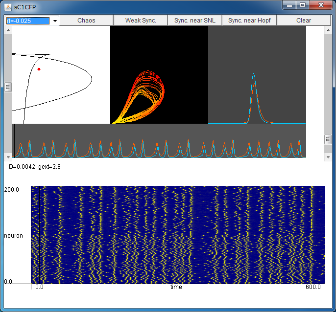
Chaos in a Pulse Neural Network :
Analysis of Synchronization with the Fokker-Planck Equation

After downloading sc1cfp.jar, please execute it by double-clicking, or typing "java -jar sc1cfp.jar".

If the above application does not start, please install OpenJDK from adoptium.net.

Explanation of Applet

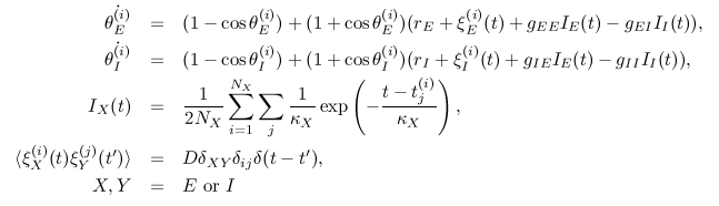
	Parameter Setting	By clicking your mouse in this field, you can change the noise intensity D (horizontal axis) and the external coupling strength g_ext (vertical axis). Synchronized firings and chaotic synchronized firings are observed depending on the values of the parameters.
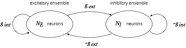
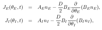
	(J_E,J_I)	Flows of probability fluxes J_E and J_I for excitatory and inhibitory ensemble are shown in the (J_E,J_I) plane. Some chaotic attractors will be observed.
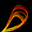
	n_E and n_I	Changes in the probability densities n_E and n_I of excitatory and inhibitory ensemble over time, are shown. Red and blue denote the excitatory and inhibitory ensemble, respectively.
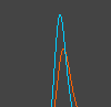
	Changes in J_E(t) and J_I(t) over time.	Changes in J_E(t) and J_I(t) over time are shown. Red and blue denote the excitatory and inhibitory ensemble, respectively. These flows correspond to the simulation with N_E=N_I=100 below.
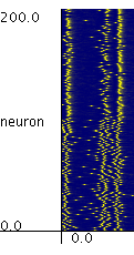
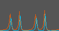
	Simulation with N_E=N_I=100	Firing times of the neurons in the system with N_E=N_I=100 are plotted. The neurons in the range from 1 to 100 are excitatory, and the neurons in the range from 101 to 200 are inhibitory neurons.

To analyze synchronization of pulse neural networks, let us consider a pulse neural network composed of excitatory neurons with internal state θ_E and inhibitory neurons with internal state θ_I that are written as

The system governed by the above equations has the form of the canonical model of slowly connected class 1 neurons. The neurons in this network are connected as the following figure.

g_int denotes the coupling strength in the ensemble, and g_ext denotes the coupling strength between two ensembles. These couplings model the synaptic coupling in the brain.

The parameters for two ensembles are r_E and r_I, respectively, and &kappa_E and &kappa_I are synaptic time constants.
The parameters are fixed as r_E=-0.025, g_int=4, κ_E=κ_I=1.

This network is a stochastic system that contains noise with intensity D. In the limit of large number of neurons, the Fokker-Planck equations for the probability densities n_E and n_I for excitatory and inhibitory ensemble, are obtained.

It is notable that asynchronous firings and synchronized firings of neurons in the network correspond to a stationary solution and a time-varying solution of the Fokker-Planck equations, respectively.

Moreover, using the Fokker-Planck equation, we can calculate probability fluxes for excitatory ensemble and inhibitory ensemble.

The probability fluxes J_E and J_I at θ_E=θ_I=π can be interpreted as the instantaneous firing rate of the excitatory ensemble and inhibitory ensemble, respectively.

With this applet, you can simulate the dynamics of the Fokker-Planck equation. The upper half of the applet shows a solution of the Fokker-Planck equation, and the lower half of the applet shows a simulation in the network with N_E=N_I=100.

By regulating the values of the parameters, you can observe various synchronized firings including chaotic ones. With the default setting, you can observe a chaotic attractor.

Particularly, the synchronized firings that are observed when you press the "Weak Sync." button, is the weakly synchronized periodic firing, in which the periodicity is observed in the average behavior of the neurons, but the periodicity of the single elementis is very weak.
Such firings may be related to the firings observed in the visual cortex or hippocampus experimentally.

Note that the number of neurons in this applet is very small (N_E = N_I = 100); therefore, the result of the simulation might differ from the results of the Fokker-Planck equation, because of the finite size effect.

This page is based on the following papers.

Takashi Kanamaru,
"Blowout bifurcation and on-off intermittency in pulse neural networks with multiple modules,"
International Journal of Bifurcation and Chaos, vol.16, no.11 (2006) pp.3309-3321. (preprint PDF)
Takashi Kanamaru,
"Analysis of synchronization between two modules of pulse neural networks with excitatory and inhibitory connections,"
Neural Computation, vol.18, no.5 (2006) pp.1111-1131. (preprint PDF)
Takashi Kanamaru and Masatoshi Sekine,
"Synchronized firings in the networks of class 1 excitable neurons withexcitatory and inhibitory connections and their dependences on the forms of interactions,"
Neural Computation, vol.17, no.6 (2005) pp.1315-1338. (preprint PDF)
Takashi Kanamaru and Masatoshi Sekine,
"An analysis of globally connected active rotators with excitatory and inhibitory connections having different time constants using the nonlinear Fokker-Planck equations,"
IEEE Transactions on Neural Networks, vol.15, issue 5 (2004) pp.1009-1017. (preprint PDF)
Takashi Kanamaru and Masatoshi Sekine,
"Analysis of globally connected active rotators with excitatory and inhibitory connections using the Fokker-Planck equation,"
Physical Review E, vol.67, no.3 (2003) 031916. (preprint PDF)

<< Analysis of Synchronization in Pulse Neural Networks with Phase Response Function / Stochastic Synchrony of Chaos in a Pulse Neural Network with Electrical Synapses >>

Introduction to Chaos and Nonlinear Dynamics