Stochastic Synchrony of Chaos in a Pulse Neural Network with Electrical Synapses


After downloading ssync.jar, please execute it by double-clicking, or typing "java -jar ssync.jar".

If the above application does not start, please install OpenJDK from adoptium.net.


Explanation of Applet

Parameter Setting 
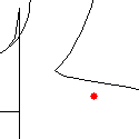
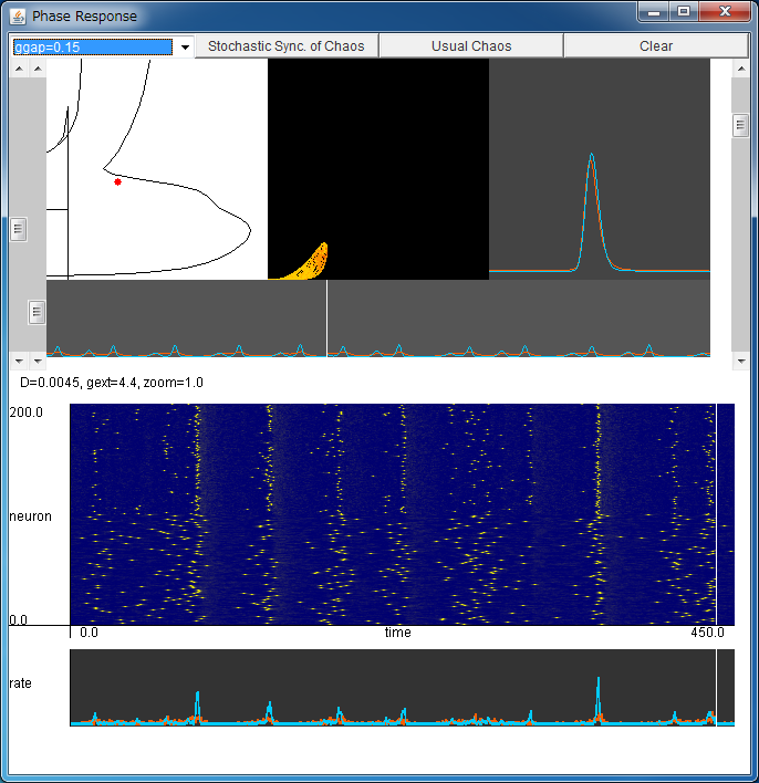
By clicking your mouse in this field, you can change the noise intensity D (horizontal axis) and the external coupling strength gext=gEI=gIE (vertical axis).
Synchronized firings and chaotic synchronized firings are observed depending on the values of the parameters. The values of the parameters can be regulated using two left scroll bars.
(JE,JI) 
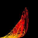
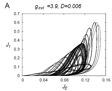
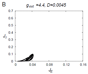
Flows of the ensemble-averaged firing rates JE and JI for excitatory and inhibitory ensemble are shown in the (JE,JI) plane.
Various forms of chaotic attractors would be observed.

You can zoom in/out using the right scroll bar.
(nE,nI) 
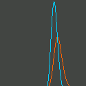
Temporal changes in the probability densities nE and nI of excitatory and inhibitory ensemble, are shown.
Red and blue denote the excitatory and inhibitory ensemble, respectively.
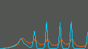
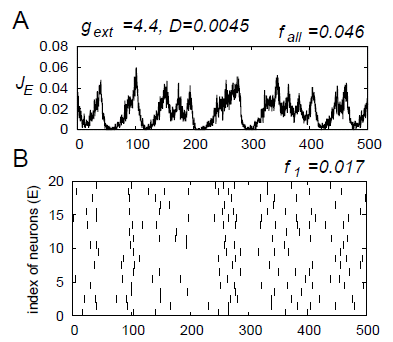
Temporal changes in JE(t) and JI(t). Temporal changes in JE(t) and JI(t) are shown.
Red and blue denote the excitatory and inhibitory ensemble, respectively.
These flows correspond to the simulation with NE=NI=100 below.
Simulation with NE=NI=100 
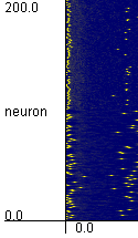
Firing times of the neurons in the system with NE=NI=100 are plotted.
The neurons in the range from 1 to 100 are excitatory, and the neurons in the range from 101 to 200 are inhibitory neurons.
The ensemble-averaged firing rates of the network with NE=NI=100 
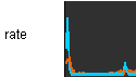
Temporal changes in the ensemble-averaged firing rates of the network with NE=NI=100.
Red and blue denote the excitatory and inhibitory ensemble, respectively.
They correspond to the above JE(t) and JI(t) which are obtained in the limit of large numbers.


Let us consider a pulse neural network composed of theta neurons written as

This network is called the canonical model of slowly connected class 1 neurons,
and it is composed of NE excitatory neurons θE and NI inhibitory neurons θI.

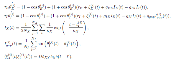
The connections IX(t) model the chemical synapses, and they give post-synaptic potentials only when the presynaptic neuron fires.

Moreover, among inhibitory neurons, this network has connections Igap(t) with electrical synapses which are realized by the structures called gap junctions, in order to incorporate the experimental findings that there are many gap junctions among inhibitory neurons in the cortex or hippocampus.

This network is a stochastic system which has noise with intensity D. In the limit of large number of neurons, the Fokker-Planck equation for the probability densities nE and nI for excitatory and inhibitory ensembles, respectively, is derived, and we can analyze the ensemble-averaged dynamics of the network using this Fokker-Planck equation.
The upper part of this applet shows the analysis of the network with the Fokker-Planck equation.

By the analysis with the Fokker-Planck equation, when the values of the parameters are appropriately chosen, this network shows a low-dimensional chaotic attractor as shown in the above figure.
The horizontal and vertical axes of this figure show the ensemble-averaged firing rate of the excitatory ensemble and the inhibitory ensemble, respectively. Such a chaotic attractor corresponds to chaotic synchronization in the network.

On the other hand, in some range of the values of the parameters, the network shows a "small" chaotic attractor as shown in the right figure. Such a "small" chaotic attractor corresponds to the phenomenon called stochastic synchrony of chaos.

Stochastic synchrony is a phenomenon where the ensemble-averaged dynamics of the network shows synchronization, but the firing rate of each neuron is very low.
In stochastic synchrony of chaos, the ensemble-averaged dynamics is chaotic, and it was discovered in our model for the first time.
A typical firing pattern of stochastic synchrony of chaos is shown in the left figure.

It is observed that the firing rate of each neuron is low, but the ensemble-averaged dynamics is chaotic.

This applet shows stochastic synchrony of chaos in the limit of large numbers (upper part), or in the system with finite number of neurons (lower part).

This page is based on the following paper.
<< Chaos in a Pulse Neural Network : Analysis of Synchronization with the Fokker-Planck Equation / Rewiring-induced Synchronization and Chaos in Pulse-coupled Neural Networks >>

Introduction to Chaos and Nonlinear Dynamics