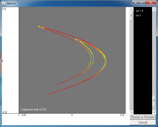
Attractor of Hénon Map
After downloading
henon.jar, please execute it by double-clicking, or typing "java -jar henon.jar".
You can expand the area by dragging the field with your mouse.
If the above application does not start, please install OpenJDK from
adoptium.net.
The definition of the Lyapunov exponent is given in the following.
First, let us define the orbital expansion rate of the Hénon map Xt+1 = F (Xt) at the point Xt+1= (xt, yt) as
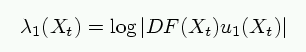
where DF(Xt) is the Jacobian matrix of the map at Xt
and u1(Xt) is a unit vector tangent to the attractor
at Xt.
Using it, the coarse-grained expansion rate is
defined as
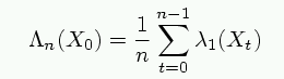
where the orbital expansion rate is averaged over n points.
The attractor of the above simulator is colored based of the value of
the coarse-grained expansion rate, and it will be explained later.
By taking the infinitely large n limit,
we can obtain the largest Lyapunov exponent as
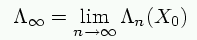
The largest Lyapunov exponent takes constant value
for almost all the initial points X0.
This simulator calculates the Lyapunov exponent
by taking the average over more than 10000 iterations.
When the size of attractor is changed, or when "Resize or Redraw" button
is pressed,
the Lyapunov exponent is re-calculated,
and this value slightly changes for each trial.
It is because the average number is finite.
Though the Lyapunov exponent does not depend on the initial point X0, the coarse-grained expansion rate does.
The attractor of the above simulator is colored based on this value.
The yellow means that the coarse-grained expansion rate is small,
and the red means large values.
In the initial condition, the value of n is 1, thus
it is identical with the orbital expansion rate.
At the curves of the attractor, the orbital expansion rate
takes negative values, thus they are colored with yellow.
And the sharp area of the attractor also form a curve,
as you can see when you expand it, thus it is also yellow.
When you enlarge the value of n, the coarse-grained expansion rate
takes in the information of the attractor, and takes
various values on the attractor.
For example, please change the value of n to 5, and press the "Resize or Redraw" button.
A few yellow areas will be observed.
These points pass the curve of the attractor in the following 5 iterations.
More specially speaking, the yellow area reflects
the trajectory of the point of tangency of stable manifold and the attractor.
The stable manifold is introduced in "Attractor of Hénon map" gallery.
Thus, the statistical properties of the coarse-grained expansion rate
reflects the phase space structure of the attractor.
By the way, for large n, the coarse-grained expansion rate
is close to the Lyapunov exponent,
thus the color of attractor will be uniform.
This page is based on the following articles.
|