Reinforcement Learning for CPG-controlled Bipedal Walking
After downloading bc_rl_app.jar, please execute it by double-clicking, or typing "java -jar bc_rl_app.jar".
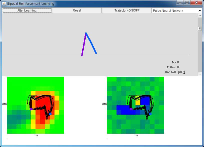
From left: Critic / Actor
By pressing "After Learning" button, parameters are set to the values
that are obtained after 500 trials.
The range of horizontal axes of critic/actor is
-1 <θ < 1, and the range of vertical axes of critic/actor is
-8.0 <ω < 8.0.
The colors of the approximated functions denote the following values.
blue: negative, green: 0, red: positive.
If the above application does not start, please install OpenJDK from adoptium.net.
Let us consider the reinforcement learning of CPG-controlled
biped walking.
The model of biped walking (Taga, 1991) is
written by an equation of motion of 14 variables
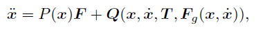 with 8 constraints.
 The position of the model is indicated by
6 variables because 14 - 8 = 6,
and they are the position (x, y) of the hip, and
the angles of hips and knees
(θR1, θR2,
θL1, θL2) for both feet.
The position of the model is indicated by
6 variables because 14 - 8 = 6,
and they are the position (x, y) of the hip, and
the angles of hips and knees
(θR1, θR2,
θL1, θL2) for both feet.
Moreover, by considering their time-derivatives
(vx, vy) and
(ωR1, ωR2,
ωL1, ωL2),
the state of this dynamical system can be described.
The torque T given to this model is determined by PD control scheme,
and the destination angles θd
are determined by Central Pattern Generator (CPG),
which is utilized in the motion control by biological systems.
In this work, as CPG, you can choose between
the ensemble-averaged firing rates
of pulse neural network proposed by Kanamaru (2006) and
the outputs of coupled van der Pol oscillators.
Based on Matsubara (2005),
let us consider the reinforcement learning of CPG-controlled
biped walking with the following scheme.
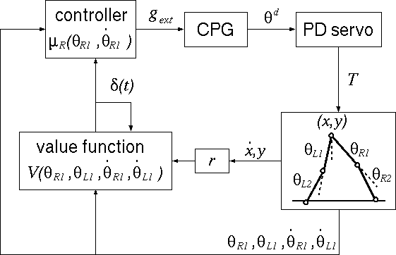
For the output of the controller, we choose the connection
strength gext of the pulse neural network.
The reward r is defined
so that the system receives a maximal reward
when both the height of the hip and the horizontal velocity are
constant.
The cumulated future reward following the policy π is defined as
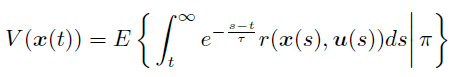 and we assume V can be written by four variables
(θR1, θL1,
ωR1, ωL1).
and we assume V can be written by four variables
(θR1, θL1,
ωR1, ωL1).
By searching large values of V(θR1, θL1,
ωR1, ωL1),
the model obtains the bipedal walking.
However, V(θR1, θL1,
ωR1, ωL1) is an unknown function,
so we must perform a function approximation to obtain
V(θR1, θL1,
ωR1, ωL1).
It is known that V(θR1, θL1,
ωR1, ωL1) can be approximated correctly
by minimizing the temporal difference (TD) error.
 The unit that approximates V(θR1, θL1,
ωR1, ωL1) is called critic.
The unit that approximates V(θR1, θL1,
ωR1, ωL1) is called critic.
On the other hand, the unit which determines the control input
is called "actor", and this is also determined by
a function approximation.
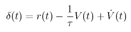
In this applet, for the learning of the critic,
we use TD(λ) method for continuous time and space,
and, for the learning of the actor, we use policy gradient method.
To apply the above method to the control of the real robot,
various simplifications were applied to the algorithm (unpublished yet).
This page is based on the following papers.
- [As for the used CPG]
Takashi Kanamaru,
"Analysis of synchronization between two modules of pulse neural networks with excitatory and inhibitory connections,"
Neural Computation, vol.18, no.5, pp.1111-1131 (2006). (preprint PDF)
Takashi Kanamaru,
"van der Pol oscillator", Scholarpedia, 2(1):2202.
- [As for the reinforcement learning for CPG-controlled bipedal walking]
T. Matsubara, J. Morimoto, J. Nakanishi, M. Sato, and K. Doya
"Learning CPG-based Biped Locomotion with a Policy Gradient Method"
Robotics and Autonomus Systems, vol. 54, issue 11, pp. 911-920 (2006).
- [As for the model of bipedal walking]
G. Taga, Y. Yamaguchi, and H. Shimizu,
"Self-organized control of bipedal locomotion by neural oscillators in unpredictable environment"
Biological Cybernetics, vol. 65, pp.147-159 (1991).
- [As for reinforcement learning]
Kenji Doya
"Reinforcement Learning in Continuous Time and Space"
Neural Computation, vol.12, 219-245 (2000).
Manual Control of Bipedal Walking >>
Back to Takashi Kanamaru's Web Page