	Chaos and Fractals: Understanding the Unpredictable by Michael Thompson, FRS Dept of Applied Maths & Theoretical Physics, Cambridge Simulations are due to Takashi Kanamaru This, and others talks, will be available on: www.sekine-lab.ei.tuat.ac.jp/~kanamaru /Chaos/e/Thompson/ and www.culive.org/MichaelThompson @
	Contents Part I 1 The Clockwork Universe of Newton 2 Chaos and Fractals 3 From Mayflies to Butterflies Part II 4 Chaos in Driven Oscillators 5 Fractal Basins and Chaotic Crises 6 Concluding Remarks @
	Part I
	A Popular Introduction to Chaos Chapter 1 The Clockwork Universe of Newton 1.1 Double Pendulum: a taste of chaos (with HL) 1.2 The Quest to Predict the Future 1.3 Newton's Principia 1.4 Newton's Impact in Poetry and Art 1.5 Newton's Impact on Philosophy 1.6 The Clockwork Universe 1.7 The Simple Pendulum 1.8 Phase Space 1.9 Dissipation makes Attractors @
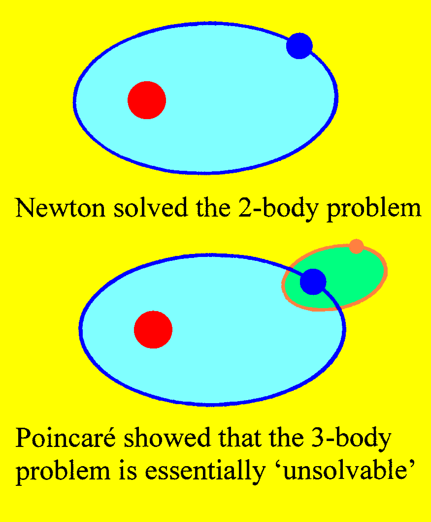
	1.1 Double Pendulum: a quick taste of chaos In mechanics, Newton's Laws allow precise analytical solutions to two problems: The simple pendulum The Sun-Earth (two body system) One small increase in complexity gives the following, with chaos and no such solution: The double pendulum The Sun-Earth-Moon (three body system) Click for double pendulum simulation @ d-pend
	1.1 (a) Double Pendulum (continued) This system conserves energy It is not dissipative Motions just continue, and do not settle Depending on the start it can exhibit: Regular oscillatory motion (upper left) Irregular chaotic motion (upper right, and lower) Click for Experiments E2 Double Pend (srb), 3m44s (2/3) @
	1.2 The Quest to Predict the Future Human beings have always sought to understand the working of nature Early in this search, astronomy proved to be a fertile field Early civilizations devised calendars to predict the seasons on Earth, and the eclipses of the sun and moon in the sky @
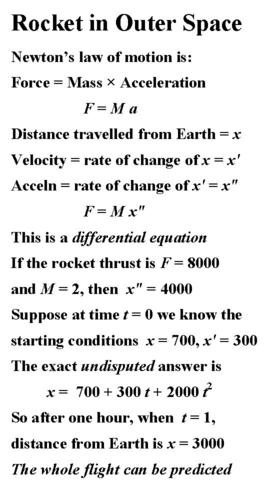
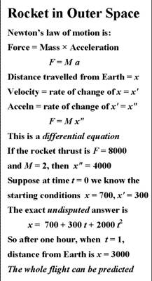
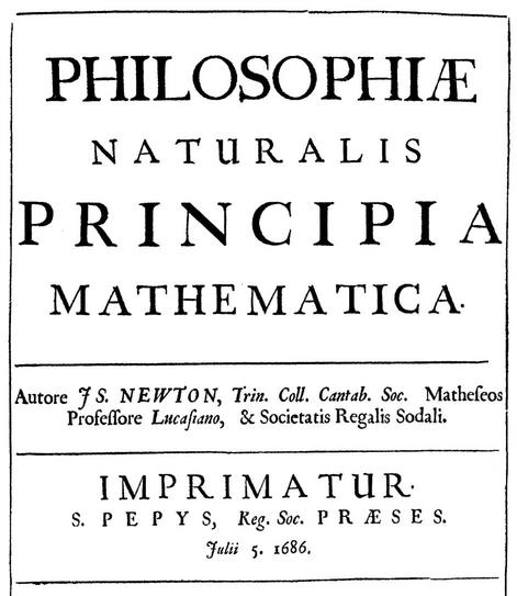
	1.3 Newton's Principia In the year 1686, Newton's Laws of Motion revolutionised science They generate a dynamical system governed by a differential equation This is still the ideal way to model a system that evolves in time Given the starting conditions, a unique future can be predicted @
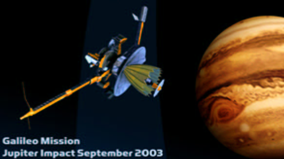
	1.3 (a) Newton's Principia (cont) Today, Newton's Laws are used throughout science and engineering In, for example, the design, the trajectory calculations, and the guidance of the Mars missions They are superseded at the sub-atomic level by quantum mechanics: and at speeds near that of light, or at cosmic distances, by relativity theory @
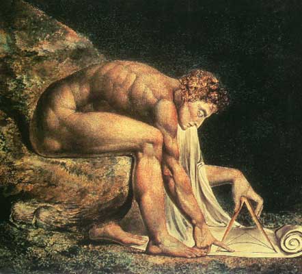
	1.4 Newton's Impact in Poetry and Art Alexander Pope wrote: Nature and Nature's laws lay hid in night: God said, Let Newton be! and all was light Blake depicted him with divider and scroll @
	1.5 Newton's Impact on Philosophy Suppose the Universe is made up of particles of matter interacting according to Newton's laws Then it is a dynamical system, governed by a (very large!) set of differential equations Given the starting positions and velocities of all particles, there is a unique outcome This type of argument was a bombshell to scientists and philosophers Pierre Laplace (1749-1827), a leading French mathematician, wrote extensively about the clockwork universe @
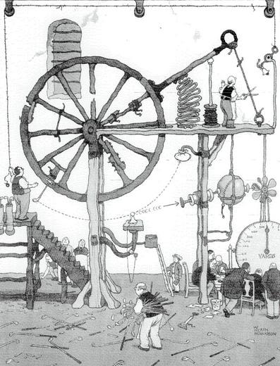
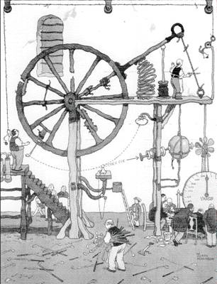
	1.6 The Clockwork Universe Newton's Laws suggested that the Universe has the predictability of a machine Golf club testing by Heath Robinson @
	1.7 The Simple Pendulum The pendulum is a classical example of a dynamical system During a church service, Galileo pondered the constant oscillation of a lamp swinging in the breeze Used for centuries in clocks, it is the very essence of regularity and predictability Click for simulation Harm @
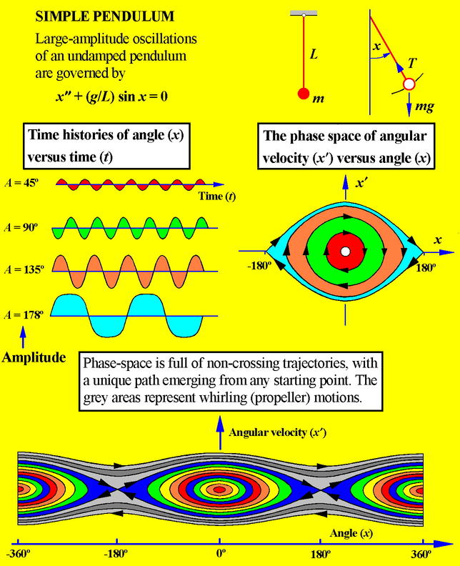
	1.8 Phase Space Phase space is the space of the starting conditions It is full of non-crossing trajectories A motion, started at any point, has a unique path Phase space of a simple pendulum is in 2D Phase space of a double pendulum is in 4D Complex systems have hundreds of dimensions @
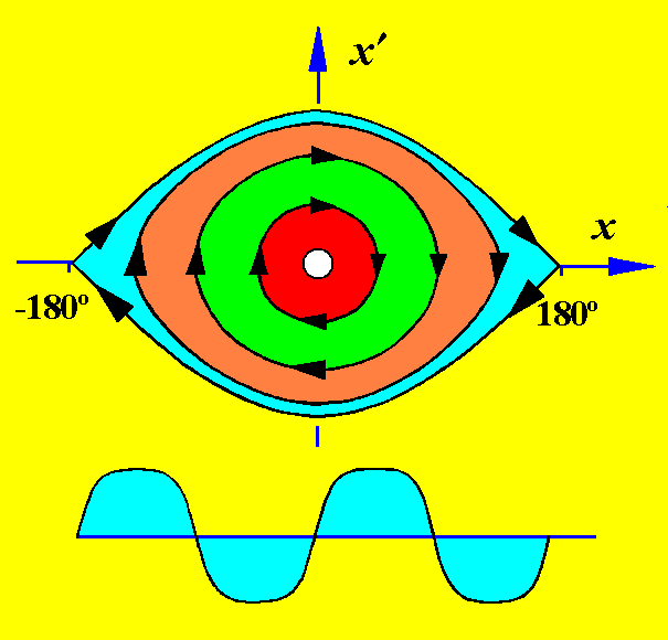
	1.8 (a) Phase space (cont) The homoclinic orbit is the creator of chaos Imagine a very small number, E (say 1/1000000000) Release the pendulum at rest, and almost exactly upside-down, but just E degrees off the vertical For years it will very slowly gather speed Today it will make a rapid transit of about 360º Then for years it will slow down, coming to rest at E degrees on the other side of the vertical If disturbed, it may or may not get over the top @
	1.8 (b) Phase space (cont) In a double pendulum the top pendulum effectively disturbs the bottom one A mechanism for chaos is: the repeated passage near an unstable state + a regular disturbance @
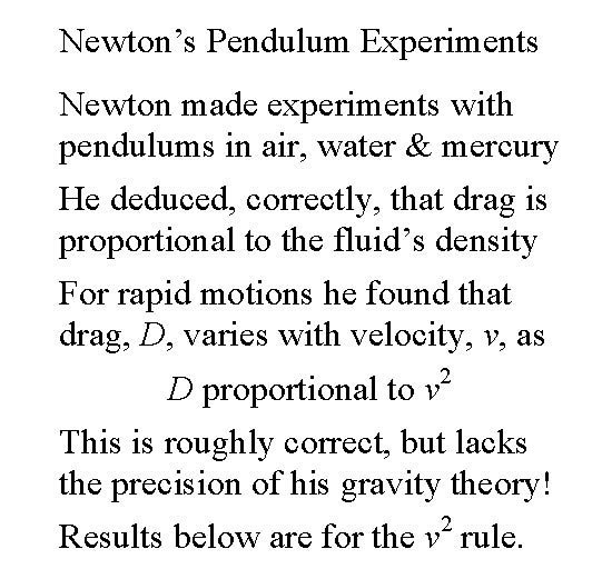
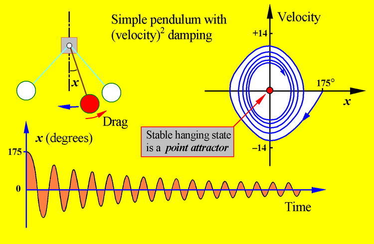
	1.9 Dissipation makes Attractors The pendulum that we have been discussing is not realistic! It oscillates for ever, with no decay of its swinging amplitude The mathematical model that we used was incomplete We ignored friction in the bearing and air-drag on the bob Both of these dissipate energy and slow the pendulum down Newton made experiments to estimate the drag force Damping changes closed orbits into spirals to a point attractor @
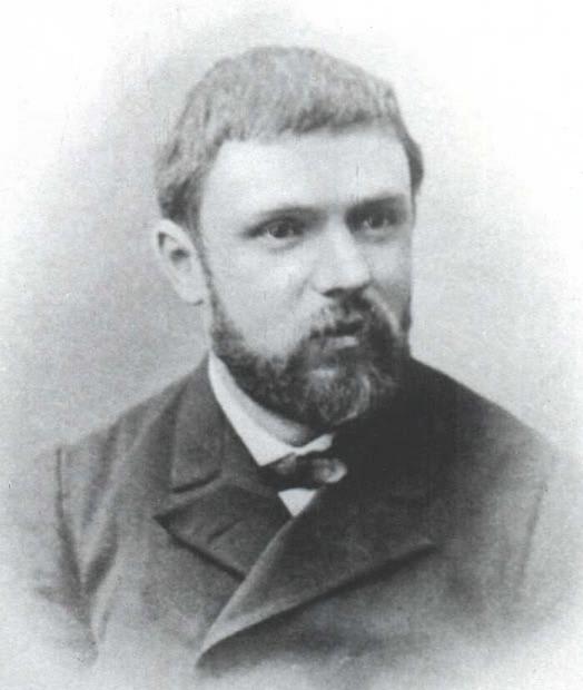
	Chapter 2 Chaos and Fractals 2.1 Henri Poincare 2.2 Lorenz Chaos (with HL) 2.3 Folding and Mixing 2.4 Rossler's Folding Band (with HL) 2.5 Poincare Section 2.6 Henon Map (with HL) 2.7 So what is a Fractal? 2.8 The Fractal Mandelbrot Set (with HL) 2.9 Another Fractal: Coastline of Britain @
	2.1 Henri Poincare Birth of Chaos Theory In 1887 the King of Sweden offered a prize to the person who could answer the question "Is the solar system stable?" Poincare, a French mathematician, won the prize with his work on the three-body problem He considered, for example, just the Sun, Earth and Moon orbiting in a plane under their mutual gravitational attractions Like the pendulum, this system has some unstable solutions Introducing a Poincare section, he saw that homoclinic tangles must occur These would then give rise to chaos and unpredictability @
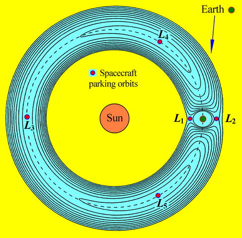
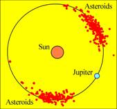
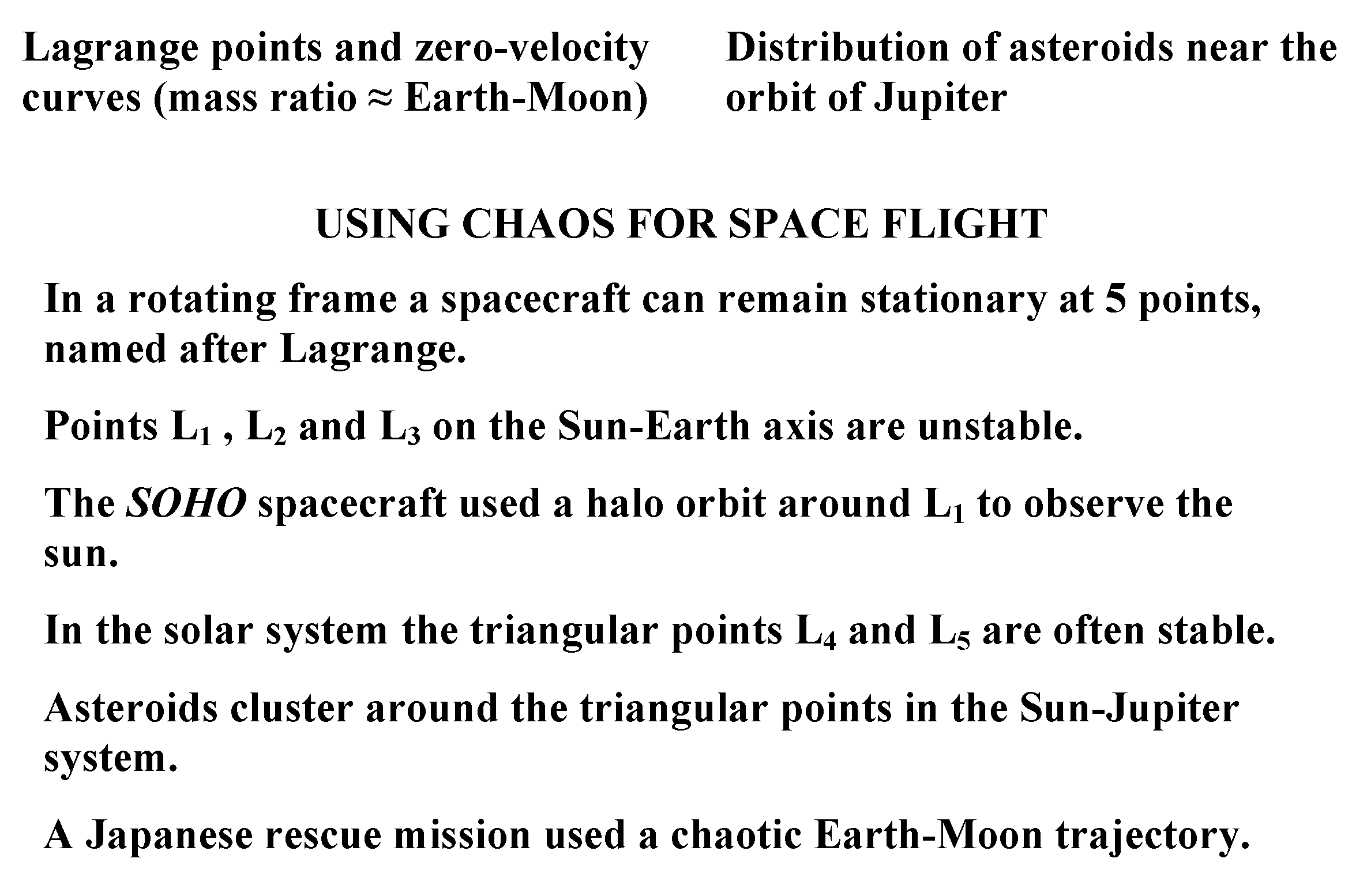
	2.1 (a) Poincare (cont) Using chaos today Rich dynamics of a chaotic state often allow it to be easily controlled Chaos is used by rocket scientists to minimise the fuel needed for a mission To save Earth from destruction by an asteroid, it could be deflected while in a chaotic regime @
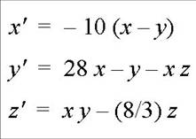
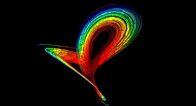
	2.2 Lorenz Chaos In 1963 Lorenz was trying to improve weather forecasting Using a computer, he discovered the first chaotic attractor Three variables (x, y, z) define convection of the atmosphere Changing in time, these variables give a trajectory in a 3D space From all starts, trajectories settle onto a strange, chaotic attractor Right and left flips occur as randomly as heads and tails Prediction is impossible Click for simulation lorenz @
	2.2 (a) Lorenz Chaos (continued) This is a very simple system of equations with dissipation Like the damped pendulum, motions settle, but here to the chaotic attractor shown This could not have been discovered without the computers that appeared in the 1960s Since the solution is chaotic, it cannot be written down in any formula In a mathematical sense the problem is unsolvable All the computer does is solve the equations in an approximate way @
	2.3 Folding and Mixing There is no crossing in phase space: so how do complex chaotic motions arise? The answer is by divergence, folding and mixing (possible with nonlinearity and 3D) @
	2.4 Rossler's Folding Band In 1976 Rossler devised a simple system to display the folding and mixing of chaos Like Lorenz, this was a set of 3 first-order autonomous differential equations Autonomous means there is no external forcing (time does not appear explicitly) In the 3D phase space the repeated folding is like making flaky pastry This creates an infinite number of infinitely thin layers: a fractal structure Click for simulation ross @
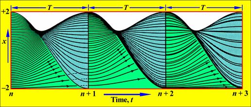
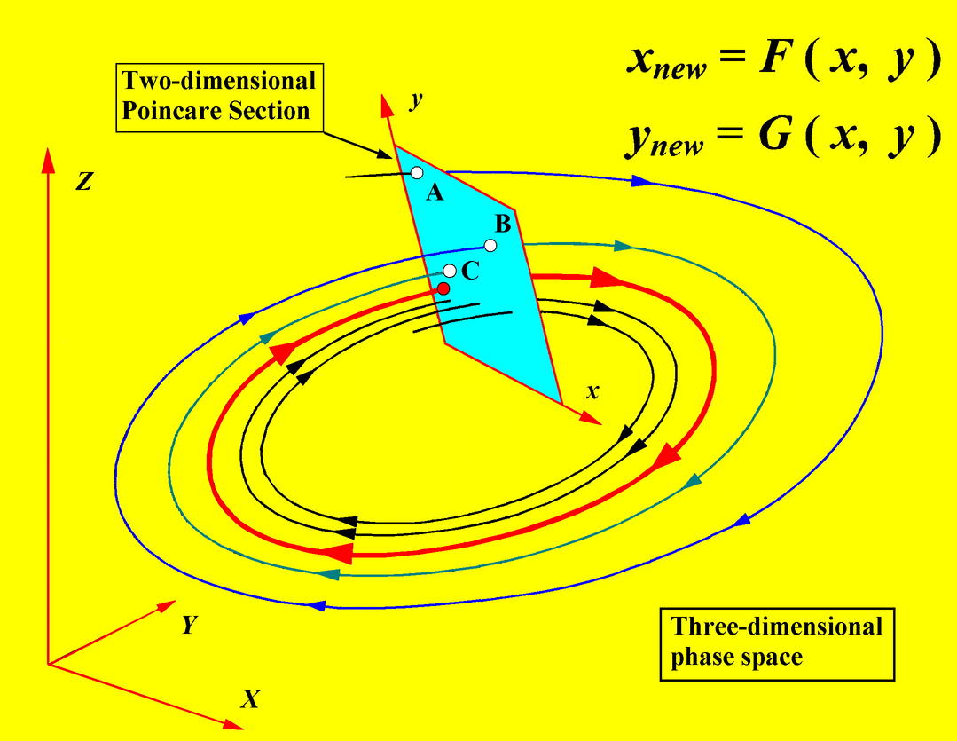
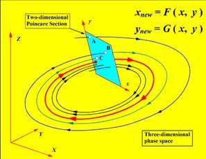
	2.5 Poincare Section To examine chaos, Poincare used the idea of a section This cuts across the phase-space orbits The original system flows in continuous time On the section, we observe steps in discrete time The flow is replaced by what is called an iterated map The dimension of the phase-space is reduced by one @
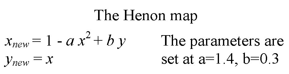
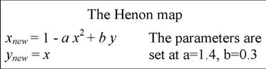
	2.6 Henon Map To show what a Poincare section of chaos would look like, Henon devised a simple 2D map Given any starting point, this map generates a sequence of points settling onto a chaotic attractor In the simulation, we will now make repeated enlargements of the attractor to see its fractal nature Click for simulation henon @
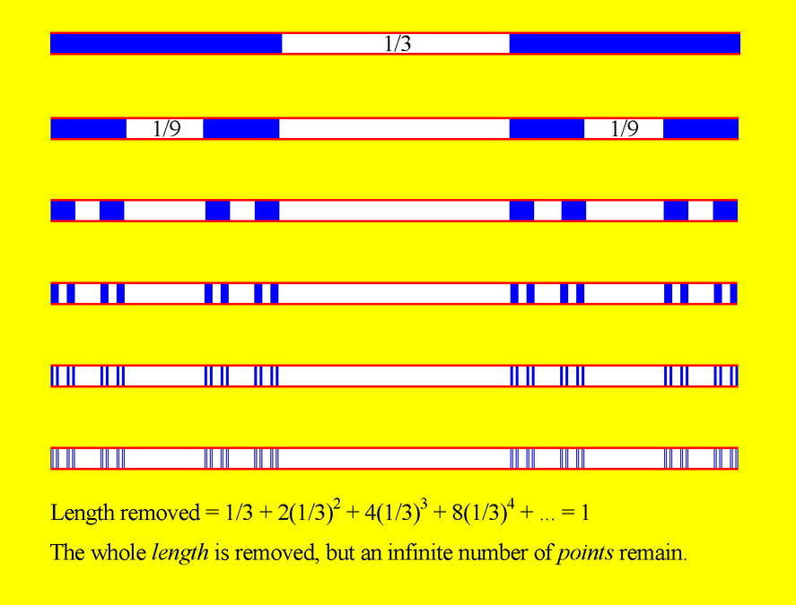
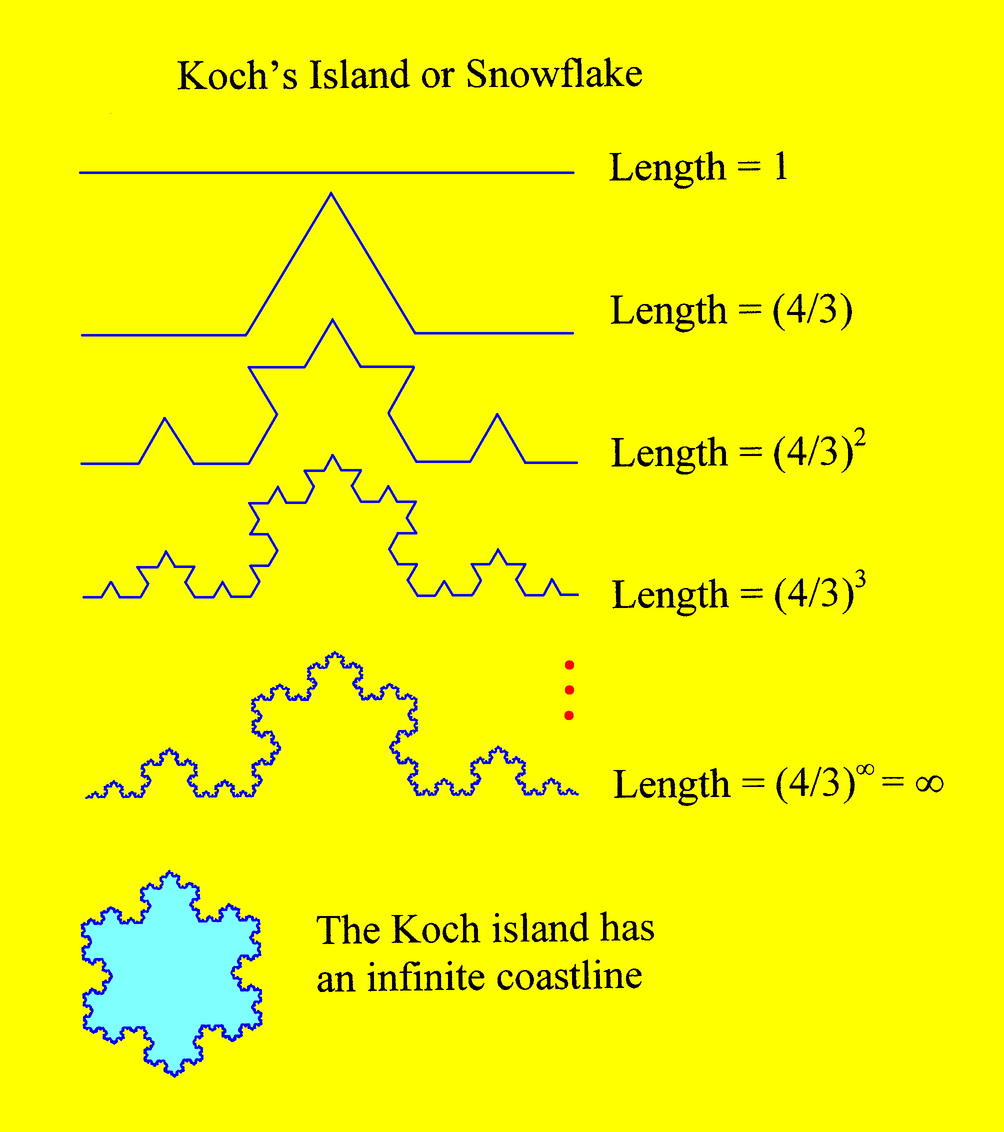
	2.7 So what is a Fractal? The simplest fractal is the Cantor set Start with a line and take out the middle-third Then take out the middle-third of the remaining lines Repeat this process for ever, to get the Cantor dust !! A sheet has dimension D=2, a line has D=1, a point has D=0 The Cantor set has the fractional value D=0.6309... @
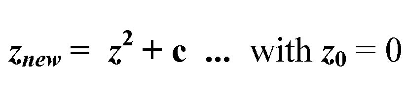
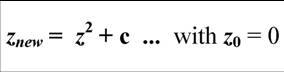
	2.8 The Fractal Mandelbrot Set Here z and c are complex numbers (with real & imaginary parts) For some values of c, the trajectory will diverge to infinity For others, it will converge (to fixed points, chaotic orbits, etc) Values of c giving convergence constitute the Mandelbrot set We view a plane whose axes are the real & imaginary parts of c The set itself will be coloured black Other points are coloured, depending on the rate of divergence Mathematically, the sequence of shrinking patterns never ends !! Click for simulation mand @
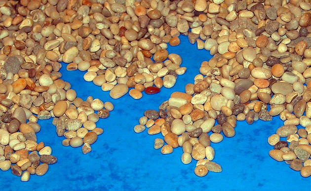
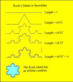
	2.9 Another Fractal: Coastline of Britain The more detailed a map, the greater is the length estimate of a coastline On the coast itself, a string would wind around every puddle, stone, crack and molecule To a good approximation the coastline is a fractal Using a divider of length A, the coastline tends to infinity as A goes to zero @
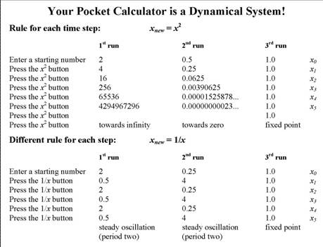
	Chapter 3 From Mayflies to Butterflies 3.1 Population Growth 3.2 Chaos in Logistic Map (with HL) 3.3 Lorenz's Butterfly 3.4 Parable of Chaos 3.5 Logistic Cascade to Chaos (with HL) 3.6 Do some Dynamics at Home 3.7 Take a break!! @
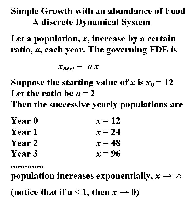
	3.1 Population Growth In ecology we use a map for yearly steps between breeding seasons The more mayflies in a pond, the more offspring we expect next year A population that increases by a fixed ratio each year will explode! Applied to humans this result alarmed Thomas Malthus His Principle of Population (1798) influenced Darwin's thoughts on natural selection @
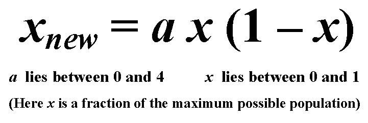
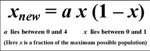
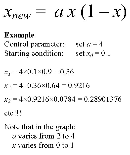
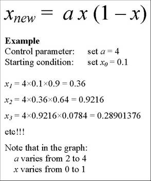
	3.2 Chaos in Logistic Map An improved mathematical model of population growth is the Logistic Map The extra factor (1 - x) recognises the constraint of limited food supplies, etc The current President of the Royal Society is Lord (Robert) May In 1976 he showed in the journal Nature how the logistic map gives rise to Chaos! The future is unpredictable due to the sensitivity to initial conditions: THE BUTTERFLY EFFECT !!! Click for simulation log @
	3.2 (a) Chaos in the Logistic Map (continued) Simple systems can have very complex behaviour This should be taught in schools!! Unfortunately text books concentrate on solvable problems, usually linear (small amplitude) ones Why did it take 300 years from Newton to chaos? (1) There were no computers (2) Researchers were looking for order (3) Random results were thought to be wrong: so they ended up in the waste paper basket @
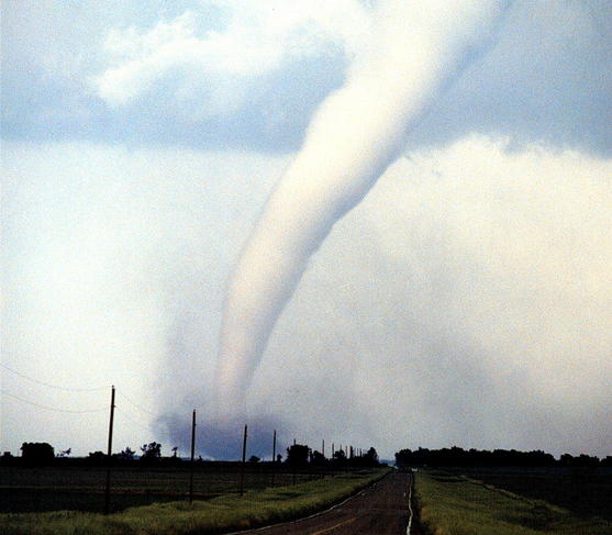
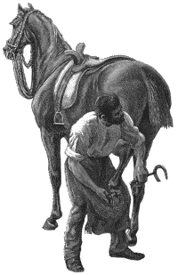
	3.3 Lorenz's Butterfly The flap of a butterfly's wings in Brazil can set off a tornado in Texas This is a parable about sensitive dependence on initial conditions A tiny difference is amplified until two outcomes are totally different Due to inevitable chaos, long term weather forecasting is impossible For want of a nail, the shoe was lost! @
	3.4 Parable of Chaos For want of a nail the shoe was lost. For want of a shoe the horse was lost. For want of a horse the rider was lost. For want of a rider the battle was lost. For want of a battle the kingdom was lost. And all for the want of a horseshoe nail. (Benjamin Franklin) @
	3.5 Logistic Cascade to Chaos The Logistic map applies the top equation repeatedly Steady state results are plotted as x against a A Feigenbaum cascade of bifurcations leads to chaos All cascades have smaller cascades within them The complex fractal pattern shrinks indefinitely Click for simulation bif @
	3.6 You can Easily do some Dynamics at Home! The Logistic map is easily programmed on a PC @
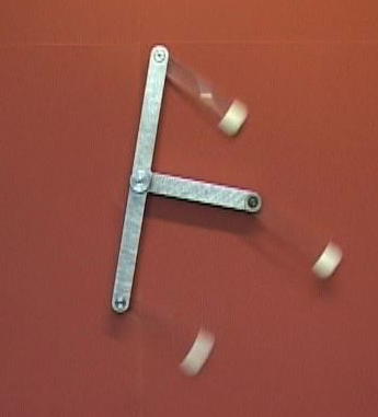
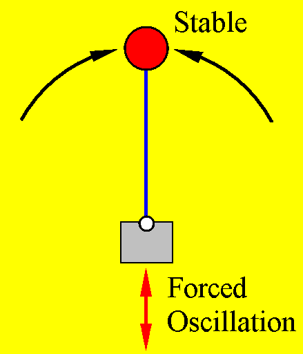
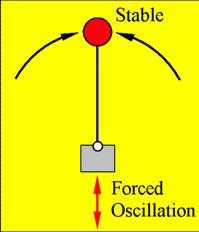
	3.7 Take a break !! I am reminded of a cartoon by Gary Larson in which a schoolboy in class is saying "Please Sir May I be excused My brain is full" After the break, in Part II of the talk we see the amazing balancing of a pendulum mounted on a jigsaw as shown above. End of Part I @
	Chaos and Fractals: Understanding the Unpredictable by Michael Thompson, FRS Dept of Applied Maths & Theoretical Physics, Cambridge Simulations are due to Takashi Kanamaru Click (forc2) This, and others talks, will be available on: www.sekine-lab.ei.tuat.ac.jp/~kanamaru /Chaos/e/Thompson/ and www.xScite.com/MichaelThompson @
	Contents Part I 1 The Clockwork Universe of Newton 2 Chaos and Fractals 3 From Mayflies to Butterflies Part II 4 Chaos in Driven Oscillators 5 Fractal Basins and Chaotic Crises 6 Concluding Remarks @
	Part II
	Introductory Experiment The Traffic Cop is a system of pendulums that illustrates in a dramatic and amusing way the surprises and complexities of chaotic motion Click for Experiments E3 Traffic Cop (srb), 3m23s (0) @
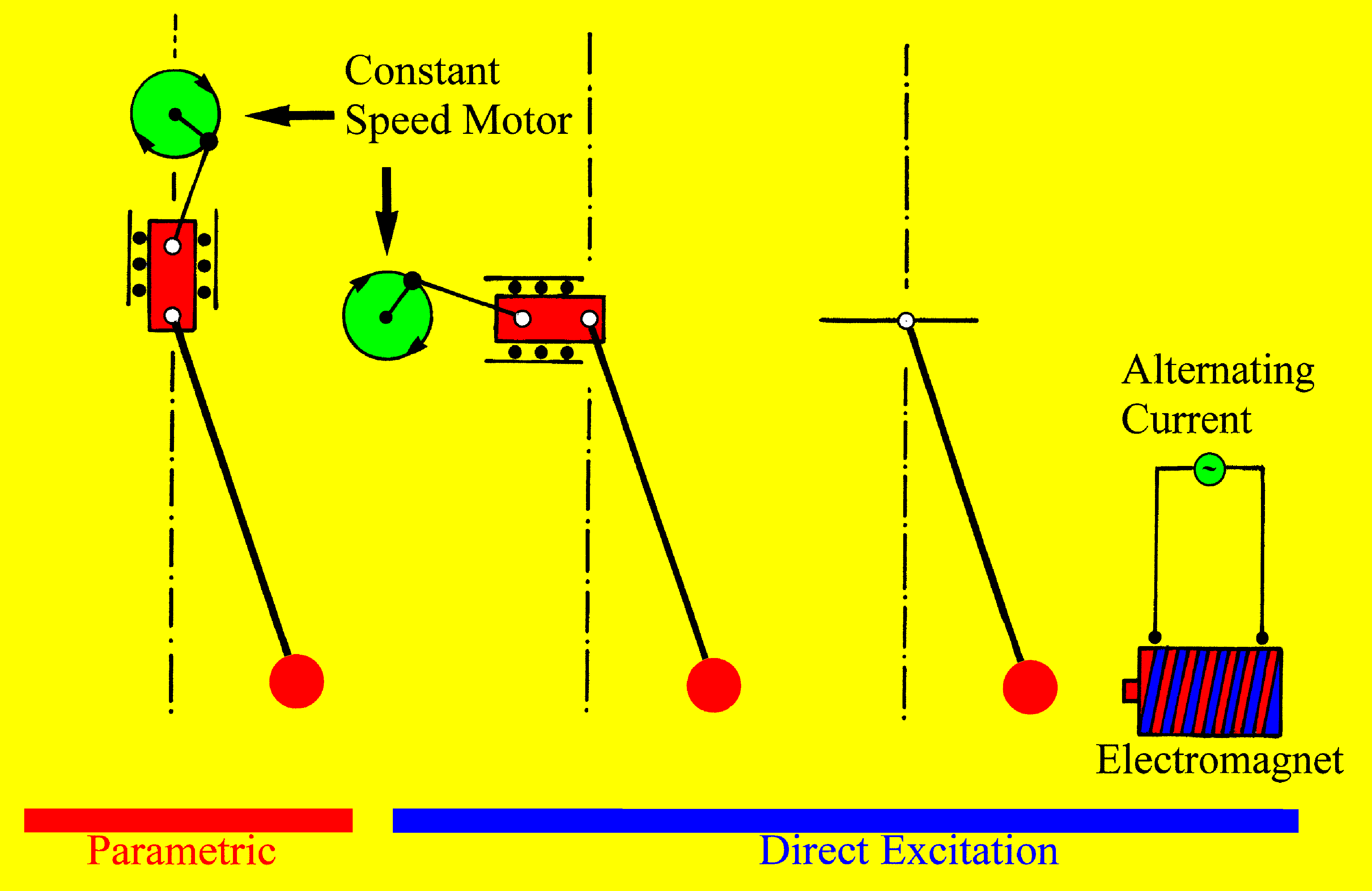
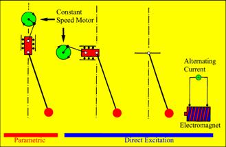
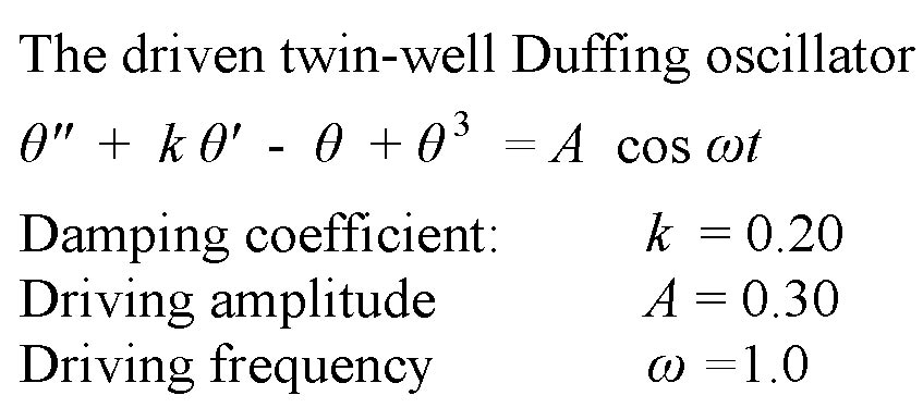
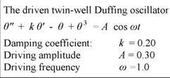
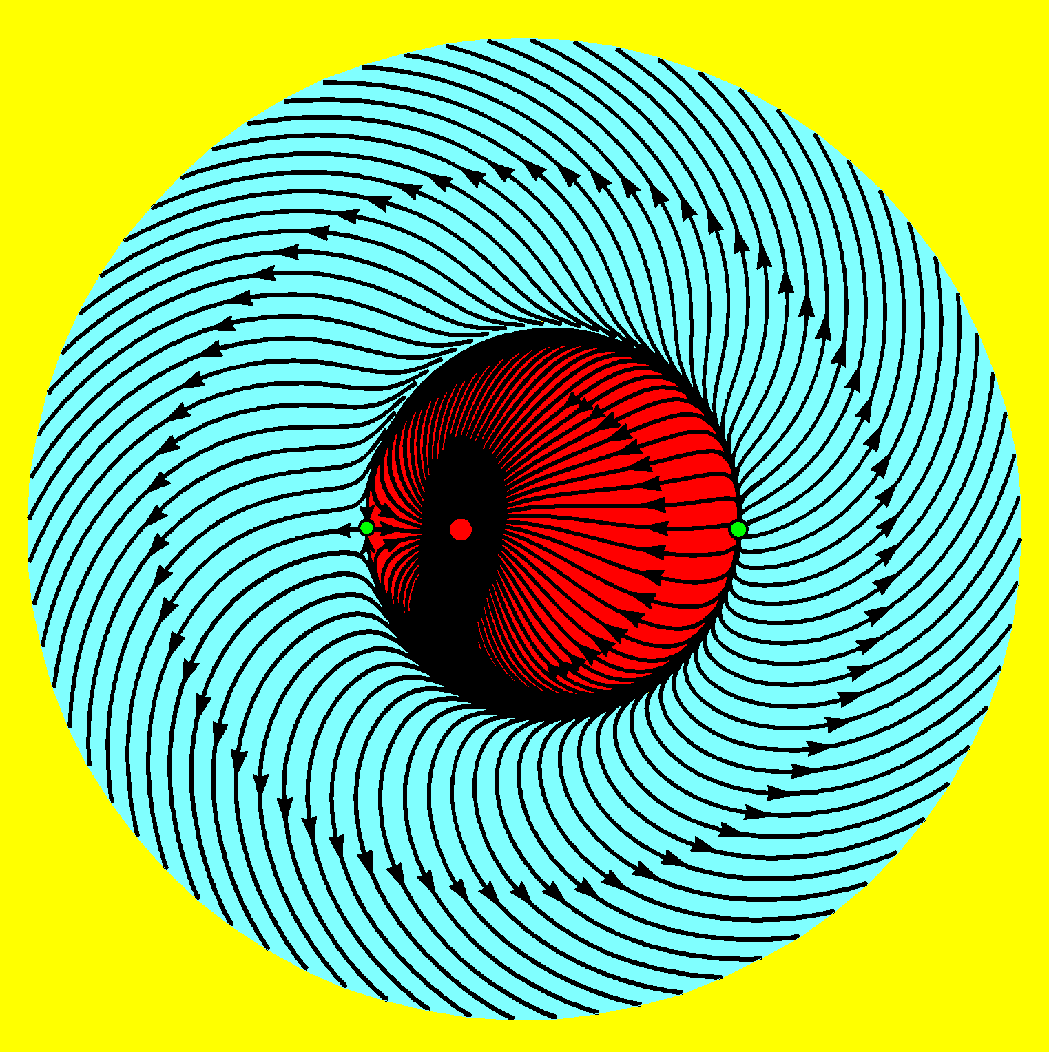
	Chapter 4 Chaos in Driven Oscillators 4.1 Some Driven Pendulums 4.2 Stroboscopic Section 4.3 Driven Pendulum: Chaos (with HL) 4.4 Driven Pendulum: Divergence (with HL) 4.5 Twin-Well Oscillator 4.6 Twin-Well Duffing: trajectory (with HL) 4.7 Twin-Well Duffing: moving cloud (with HL) 4.8 Twin-Well Duffing: settling to attractor (with HL) @
	4.1 Some Driven Pendulums Three different ways of driving a pendulum: A simple undamped pendulum swings forever. It has closed orbits in a 2D phase space A simple damped pendulum settles to rest. Spirals lead to a point attractor in a 2D phase space A forced or driven pendulum has a 3D phase space, and can exhibit chaos @
	4.1 (a) The JigSaw Pendulum @
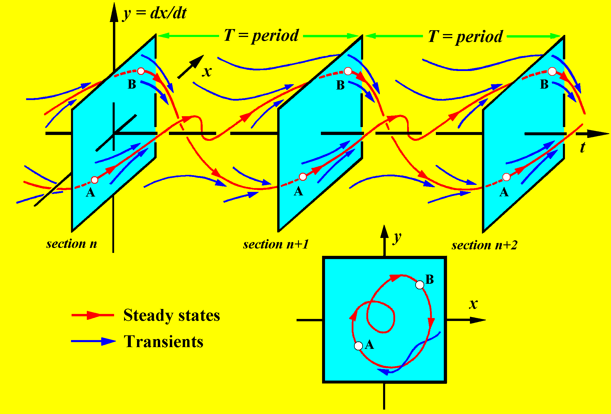
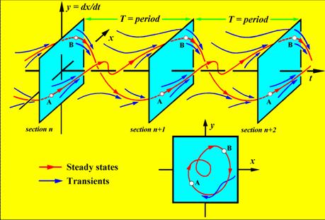
	4.2 Stroboscopic Section A driven oscillator has a 3D phase space with displacement (x), velocity (y), time (t) @
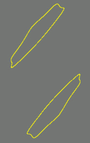
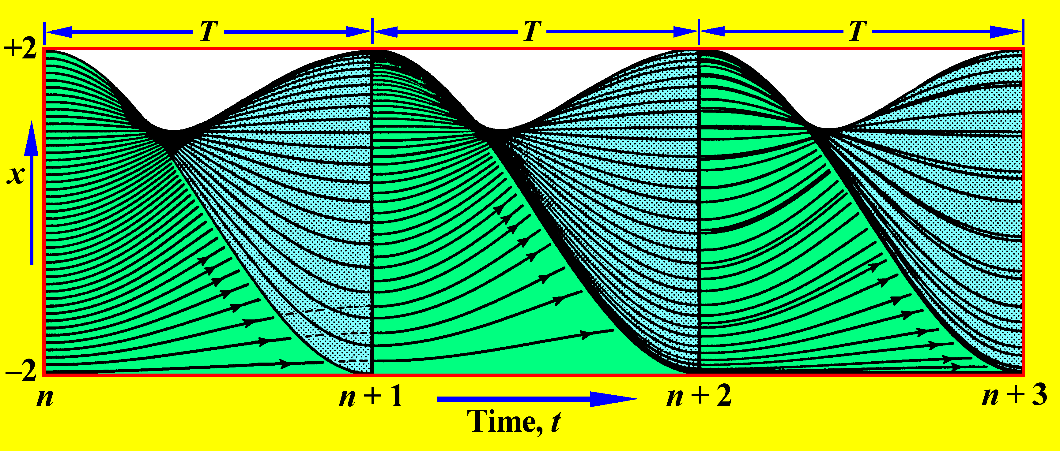
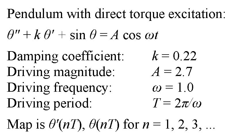
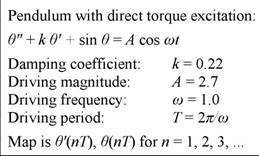
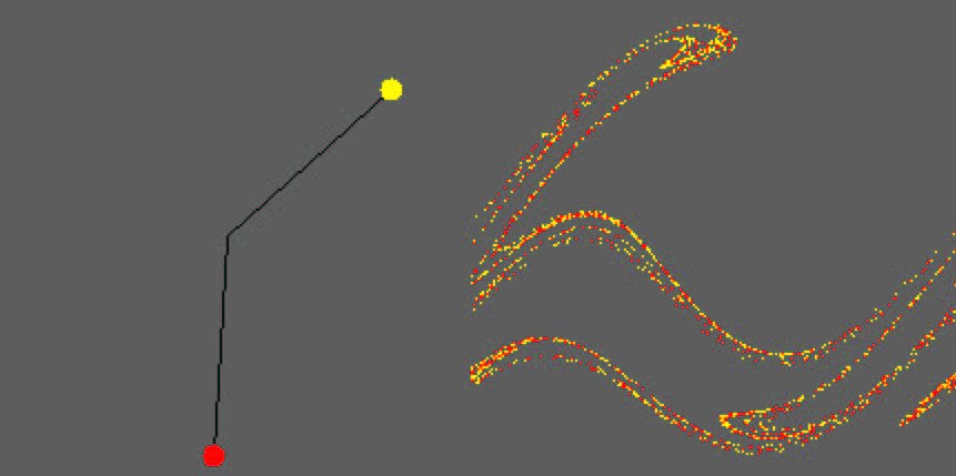
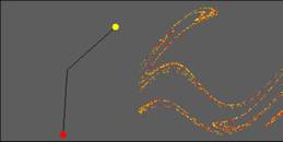
	4.3 Driven Pendulum: Chaos Chaotic tumbling of a damped and driven pendulum In a stroboscopic section a strange attractor appears The two identical pendulums have slightly different starts Their motions separate, their sections remain the same We see ORDER in CHAOS Click for simulation forc2 @
	4.4 Driven Pendulum: Divergence So how accurate is a computed trajectory? A computer solves an equation by taking short steps in time, and estimating where the system will move in each step Put bluntly, it makes a small error at each step Unfortunately chaos magnifies small errors So a computed trajectory is basically unreliable We hope that, like our pendulums, the trajectory may be wrong, but the attractor may be right Issues like this are still a research topic @
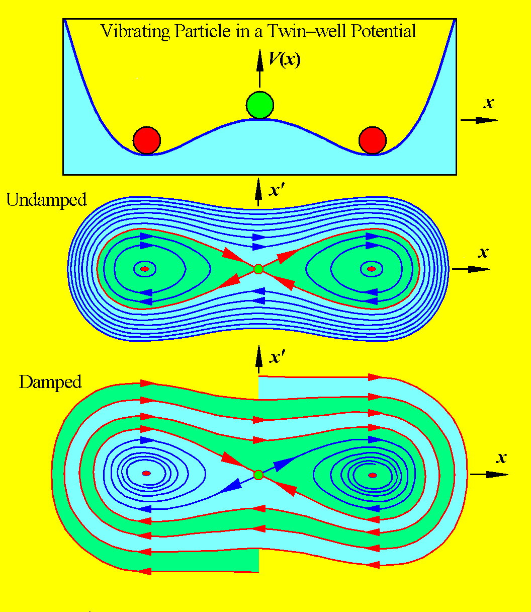
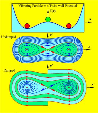
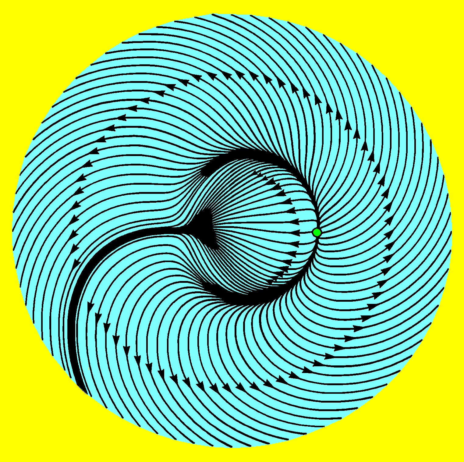
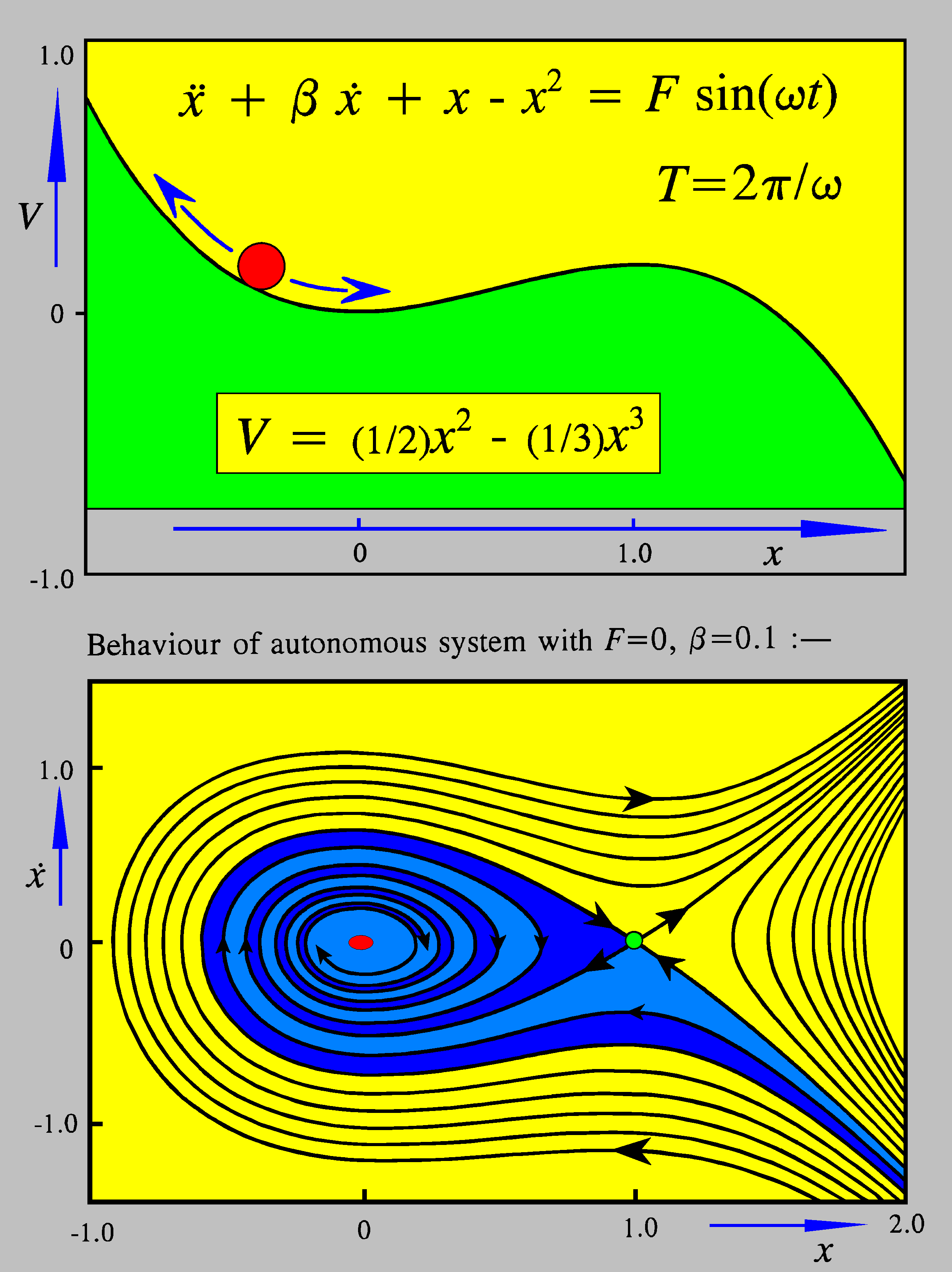
	4.5 Twin-Well Oscillator Imagine a ball rolling on the top energy surface The undamped 2D portrait has closed orbits With damping we have 2 attractors in their basins @
	4.6 Twin-Well Duffing: chaotic attractor Now imagine the ball-bearing is being pulled back and forth by a giant alternating-current electromagnet Equations like this are named after Duffing Stroboscopic sampling of the steady state gives:
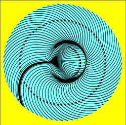
	4.7 Twin-Well Duffing: moving cloud We have seen how stroboscopic sampling gives us the familiar fractal picture of the chaotic attractor We can learn a lot about the stretching, folding and mixing of chaos by looking at intermediate sections These can be assembled into a movie, showing the distortions of the attractor as we move through time. Click for simulation cloud only (Mpeg) (all) @
	4.9 Twin-Well Duffing: settling to attractor For the damped, undriven pendulum we saw how trajectories spiral into a point attractor This point attractor is the stable hanging state of the simple pendulum We shall now see how nearby trajectories are attracted into the stable chaotic motion of the driven twin-well oscillator Click for simulation duff-transient @
	Chapter 5 Fractal Basins and Chaotic Crises 5.1 ABC of Nonlinear Dynamics 5.2 Escape from a Well 5.3 Homoclinic Tangling 5.4 Fractal Basin Erosion (with HL) 5.5 Chaos in Crisis @
	5.1 ABC of Nonlinear Dynamics Key concepts of dissipative dynamics are: Attractor Basin Catastrophe (bifurcation) @
	5.1 (a) ABC of Nonlinear Dynamics (continued) The next time you have a bath, take a good look at the soap bubbles. Imagine you are looking at a 3D phase space. Each bubble is a basin of attraction At its centre is an attractor Attractors are of just 4 types: Point attractor Periodic attractor Quasi-periodic attractor Chaotic attractor A given system can have many attractors of different types Each sits in its own basin of attraction The attractor chosen depends on the starting conditions @
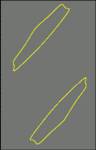
	5.2 Escape from a Well Escape from a potential well is a recurring problem in science and engineering Consider a damped particle in a well excited by a direct periodic driving force If the driving is switched off, the 2D phase portrait is as shown in the lower picture The safe basin of attraction is shown in white Starts in the grey area escape over the hilltop to infinity @
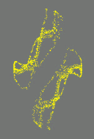
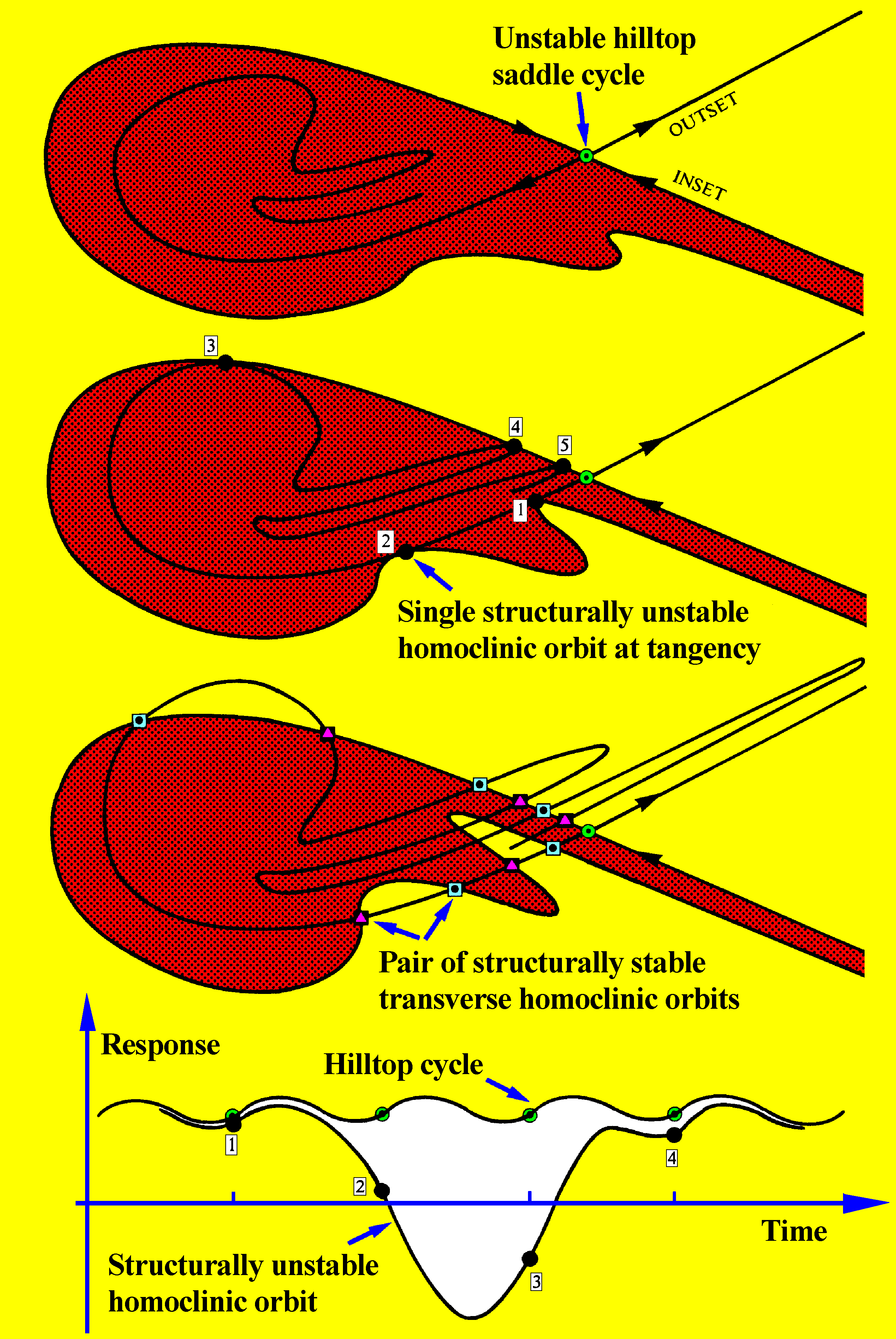
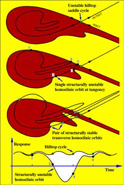
	5.3 Homoclinic Tangling (like that foreseen by Poincare in 1887) Once we start driving, the phase portrait is in 3D We must view the basin in a stroboscopic section The hill-top solution still has an inset and an outset Solutions step along these lines (unlike the flow in 5.2) As the driving increases, the inset and outset get tangled They intersect one another an infinite number of times The boundary of the safe basin becomes fractal @
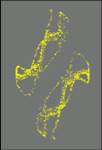
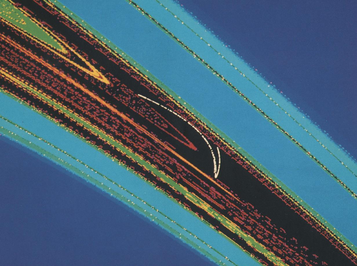
	5.4 Fractal Basin Erosion As the driving increases, fractal fingers created by the homoclinic tangling make a sudden incursion into the safe basin: the integrity of the in-well motions is lost Colours show escape time, measured in driving periods Click for Simulation (made by Prof Joseph Cusumano) Cusu 2m28s (1/2+) @
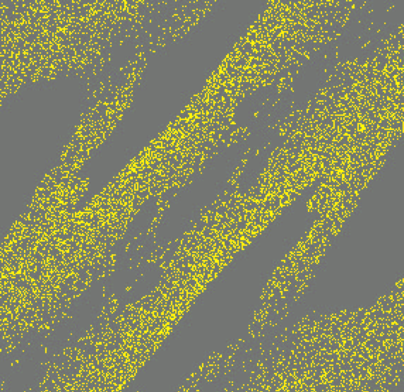
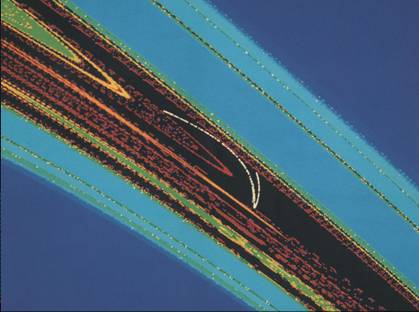
	5.5 Chaos in Crisis An ABC event that triggers escape from the well ... The white chaotic attractor is about to vanish as it collides with its fractal basin boundary At such a crisis the attractor disappears. The system jumps to a different state: ours jumps out of the well ! @
	Chapter 6 Concluding Remarks 6.1 Chaos and Mathematical Models 6.2 Properties of Chaos 6.3 Where has chaos been found or used? 6.4 Conclusion (with HL) @
	6.1 Chaos in Mathematical Models Chaos is a random output from equations which have precise deterministic rules It exhibits extreme sensitivity to initial conditions Chaotic solutions are mathematically unsolvable Computations are prone to enormous errors Detailed prediction impossible However there is order within chaos @
	6.2 Properties of Chaos The butterfly effect makes detailed prediction impossible However there is order within chaos Chaotic attractors are stable and there is no danger of a sudden excursion off the attractor An engineering system in a chaotic state is not necessarily dangerous: it might have advantages @
	6.3 Where has chaos been found or used? PHYSICS Particle accelerators Quantum mechanics Turbulence and convection Lasers, nonlinear optics ASTRONOMY and EARTH SCIENCE Gaps in the asteroid belt Tumbling of Hyperion Earth's magnetic reversals Weather and climate CHEMISTRY Atomic & molecular dynamics Pattern formation Flames and combustion Reaction kinetics BIOLOGY and MEDICINE Populations, natural selection Disease epidemics Irregularities of the heartbeat Brain rhythms ENGINEERING and ELECTRONICS Flight dynamics in air and space Capsize of ships Actuators, controls and gears Electronic circuits Communications, encryption Power supply, black-outs @
	6.4 Conclusion In this 2-Part talk we have seen just the tip of chaos theory It is said that human brains work best in a chaotic state So if your brain is in chaos, the lecture was a success! Click (brain) for simulation of chaos in a neuron For this and other talks see: www.culive.org/MichaelThompson and www.sekine-lab.ei.tuat.ac.jp/~kanamaru/Chaos/e/Thompson/ @ Back