Periodically Forced Pendulum


After downloading forced.jar, please execute it by double-clicking, or typing "java -jar forced.jar".

If the above application does not start, please install OpenJDK from adoptium.net.

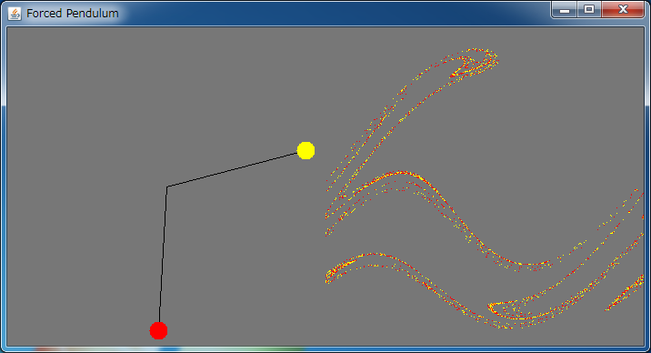
The points which show the states of pendulums are plotted in the right field every period. If you wait about 10 minutes, you can see the ordered figure.


Here we treat an oscillator called as periodically forced pendulum, governed by a differential equation,

d2θ/dt2 = - γ dθ /dt - sin(θ) + a cos(ω t),

where γ = 0.22, ω =1.0 , a = 2.7. Solving this equation by the 4th-order Runge-Kutta method numerically, the chaotic solution is obtained.
This simulator visualizes this solution as the motion of pendulums.
Two independent oscillators with different initial conditions are drawn in the same field. Because the chaotic solution is sensitive to initial conditions, these two oscillators' motions are separated from each other as time passes.
Therefore, in order to predict the future precisely, we must observe the state of the system with an infinitely high precision.
However, the theory of quantum mechanics tells us that such an observation is impossible.

When this motion is observed in the three dimensional phase space (θ, dθ/dt,t), a strange attractor appears as shown in "Periodically forced pendulum" animation.
The data (θ(nT),dθ(nT)/dt) (n=0,1,2,...) sampled every T=2 π/ω are shown in the right field of this simulator. After a while, a strange attractor will be observed.

In the simulator, it is observed that the states of yellow and red pendulums separate from each other. Actually, in the right field, it is also observed that two trajectories exists on the identical chaotic attractor.
Such a co-existence of chaos and order is a typical property of the deterministic chaos.

<< Harmonic Oscillator / Duffing Equation >>

Back to Various Pendulums

Introduction to Chaos and Nonlinear Dynamics